Renewable Energy Characterization

Overview

VerveStacks implements a comprehensive three-stage renewable energy characterization process that addresses the critical challenges of spatial resource assessment, land-use conflicts, and temporal profile generation. This methodology ensures realistic renewable energy representation in energy system optimization models while maintaining computational efficiency.

Three-Stage Renewable Characterization Process:

Land-Use Conflict Resolution: Conservative LCOE-based overlap adjustment between solar and onshore wind
Resource clustering: Dynamic spatial aggregation of the 50X50km grid cell renewable potential into clusters.
Shape Assignment: Temporal profile generation with grid vs. nogrid model differentiation

Stage 1: Land-Use Conflict Resolution

The Challenge: Avoiding Double-Counting

REZoning datasets provide separate suitable area assessments for solar and onshore wind technologies. However, these assessments often overlap significantly, leading to potential double-counting of land resources in energy system models.

LCOE-Based Overlap Adjustment Methodology

VerveStacks implements a sophisticated LCOE Share Allocation approach that resolves land-use conflicts while preserving economic rationality:

Core Algorithm:

-- For each (ISO, grid_cell) pair with both solar and wind potential:

-- 1. Calculate overlap area
overlap_area = MIN(solar_suitable_area, wind_suitable_area)

-- 2. Determine competing capacities in overlap grid cell
IF solar_area <= wind_area THEN
    solar_competing = solar_capacity  -- All solar competes
    wind_competing = (overlap_area / wind_area) * wind_capacity  -- Partial wind
ELSE
    wind_competing = wind_capacity   -- All wind competes
    solar_competing = (overlap_area / solar_area) * solar_capacity  -- Partial solar

-- 3. Calculate LCOE-based allocation shares
lcoe_sum = solar_lcoe + wind_lcoe
solar_share = wind_lcoe / lcoe_sum  -- Higher wind LCOE = more solar allocation
wind_share = solar_lcoe / lcoe_sum  -- Higher solar LCOE = more wind allocation

-- 4. Allocate competing resources
solar_final = solar_competing * solar_share + solar_untouched
wind_final = wind_competing * wind_share + wind_untouched

Key Principles:

Economic Rationality: Cheaper technology (lower LCOE) receives larger share of contested land
Conservative Approach: Reduces total renewable potential to avoid over-optimistic assessments
Technology Neutrality: No arbitrary preferences - purely data-driven allocation
Preservation of Non-Overlapping Resources: Full potential maintained where no conflict exists

Global Implementation:

The methodology processes 100+ countries simultaneously, applying identical logic to each (ISO, grid_cell) pair:

**Land-Use Adjustment Impact (Global)**
Impact Category	Before Adjustment	After Adjustment	Change (%)
Solar Generation (TWh)	125000	118750	-5.0
Wind Generation (TWh)	180000	162000	-10.0
Total Generation (TWh)	305000	280750	-7.9
Solar Capacity (GW)	45000	42750	-5.0
Wind Capacity (GW)	60000	54000	-10.0
Grid Cells Adjusted	45000	45000	0.0
ISOs Processed	195	195	0.0

Note: Typical reductions of 5-15% in total renewable potential ensure conservative, realistic resource assessments.

Stage 2: Renewable Resource Clustering

Intelligent Spatial Aggregation

After land-use adjustment, VerveStacks transforms high-resolution renewable energy grid cells into optimized clusters that balance model complexity with geographic realism. This process converts hundreds of individual renewable energy grid cells into manageable clusters while preserving essential resource characteristics and grid connectivity patterns.

The VerveStacks Philosophy: Flexible Structures from Common Data

A core principle of VerveStacks is creating different structures from the same underlying data. Just as the platform generates multiple timeslice configurations from identical hourly profiles, renewable resource clustering produces varied spatial aggregations tailored to specific analytical needs while maintaining data consistency and methodological rigor.

Clustering Methodology

Technology-Specific Multi-Stage Pipeline

Renewable resource clustering follows a sophisticated multi-stage process performed separately for each technology:

Grid Cell Identification: Extract renewable energy grid cells from REZoning database for each technology
Resource Quality Filtering: Apply technology-specific capacity factor thresholds to exclude low-quality resources - Solar PV: Grid cells with <5% capacity factor excluded - Onshore Wind: Grid cells with <8% capacity factor excluded - Offshore Wind: Grid cells with <8% capacity factor excluded
Resource Characterization: Generate hourly capacity factor profiles using Atlite weather data for each technology independently
Grid Connectivity: Calculate distance to nearest transmission infrastructure for each grid cell (transmission buses ≥150kV)
Technology-Specific Feature Engineering: Combine technology-specific resource profiles with spatial and infrastructure data
Independent Clustering: Apply hierarchical clustering with technology-optimized feature weighting for each renewable type
Quality Validation: Assess cluster coherence and grid connectivity per technology
Separate Output Generation: Create independent timeseries files for each technology cluster set

Algorithm Details

The clustering algorithm uses hierarchical clustering with Ward linkage, optimized for renewable energy applications. Only economically viable grid cells are included in the clustering process based on capacity factor thresholds that ensure realistic renewable energy deployment potential.

Technology-Specific Clustering Approach:

VerveStacks performs separate clustering for each renewable technology to optimize resource representation and avoid cross-technology interference in cluster formation:

Solar PV clustering: Independent clustering using only solar capacity factor profiles
Wind onshore clustering: Independent clustering using only wind onshore capacity factor profiles
Wind offshore clustering: Independent clustering using only wind offshore capacity factor profiles (when applicable)

Feature Weighting (Per Technology): - Technology profiles: 50% - Temporal generation patterns for the specific technology - Grid distance: 40% - Infrastructure connectivity to transmission buses - Spatial coordinates: 10% - Geographic proximity for contiguous clusters

Dimensionality Reduction: - PCA preprocessing: Up to 50 components for each technology’s hourly profiles - Standardization: All features normalized before clustering within each technology - Distance metric: Euclidean distance in transformed feature space

Dynamic Cluster Number Determination: The number of clusters is determined dynamically based on the number of renewable energy grid cells using the formula:

n_clusters = int(np.clip(n_cells ** 0.6, 10, 300))

This scaling approach ensures: - Small countries (few grid cells): Minimum 10 clusters per technology for adequate resolution - Large countries (many grid cells): Reasonable computational complexity with maximum 300 clusters per technology - Balanced scaling: Sublinear growth prevents excessive clustering in large countries - Technology independence: Each renewable type gets optimally sized cluster sets

Benefits of Technology-Specific Clustering:

Resource Optimization: Solar and wind resources have fundamentally different temporal patterns and geographic distributions
Cluster Purity: Avoids mixing high-solar/low-wind cells with low-solar/high-wind cells in the same cluster
Grid Connection Accuracy: Each technology can connect to the most appropriate transmission infrastructure
Model Flexibility: Enables technology-specific capacity expansion and dispatch optimization
Temporal Fidelity: Preserves distinct diurnal (solar) and weather-driven (wind) generation patterns

Technology-Specific Capacity-Weighted Profile Aggregation

For each technology cluster, hourly generation profiles are computed using capacity-weighted averaging with technology-specific data:

def calculate_weighted_cluster_profiles_2(clusters, profiles, technology):
    """
    Calculate capacity-weighted cluster profiles for renewable technologies
    """
    cluster_profiles = {}
    for cluster_id in clusters:
        grid_cells_in_cluster = clusters[cluster_id]

        # Get capacity weights (MW potential)
        weights = profiles[grid_cells_in_cluster]['capacity_mw']

        # Calculate weighted average hourly profile
        weighted_profile = np.average(
            profiles[grid_cells_in_cluster]['hourly_cf'],
            weights=weights,
            axis=0
        )

        cluster_profiles[cluster_id] = weighted_profile

    return cluster_profiles

This approach ensures that grid cells with higher renewable energy potential have proportionally greater influence on the cluster’s temporal generation pattern.

Country Examples and Validation

Brazil Solar Clustering (KAN Grid)

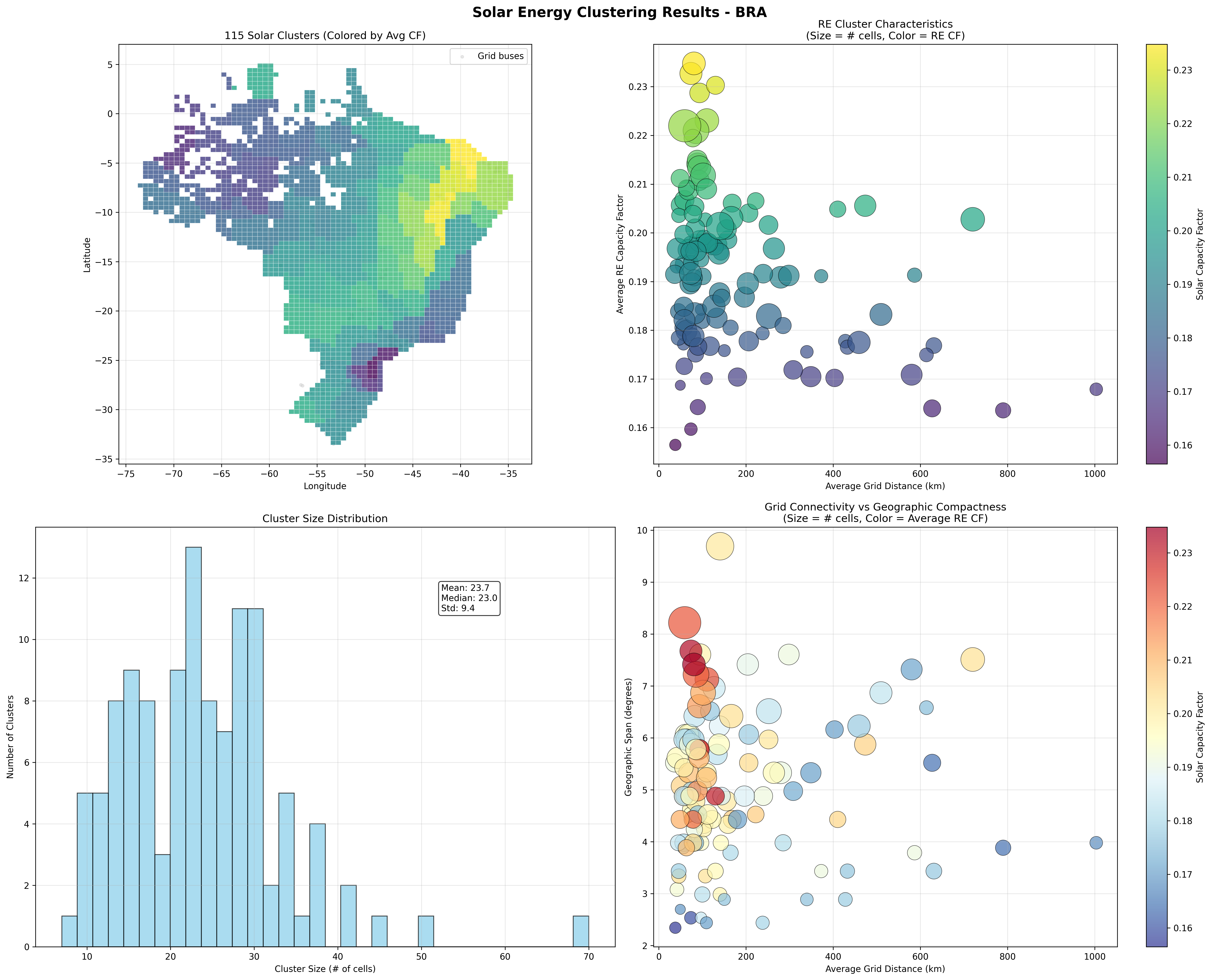
Brazil Solar Clustering Results — Brazil Solar Resource Clustering - KAN Grid Definition

3,095 renewable grid cells processed
124 clusters created (using dynamic scaling: 3,095^0.6 ≈ 124)
Average cluster size: 25.0 grid cells per cluster
Solar capacity factor: 15.6% to 23.2% range (average 19.1%)
Grid connectivity: Distance to cities (CIT grid)
Cluster size range: 6 to 69 grid cells per cluster

Brazil Offshore Wind Clustering (KAN Grid)

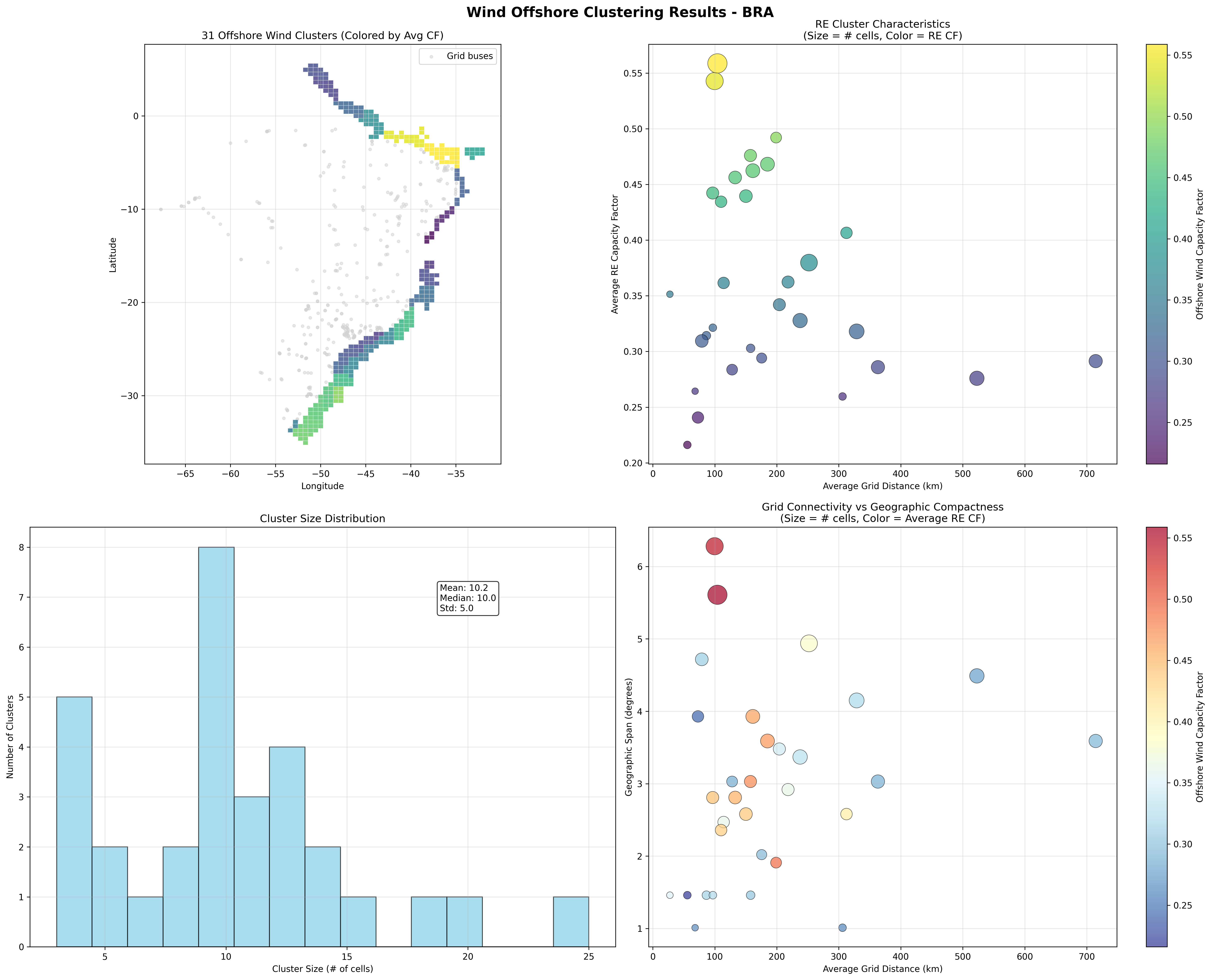
Brazil Offshore Wind Clustering Results — Brazil Offshore Wind Resource Clustering - KAN Grid Definition

1,120 renewable grid cells processed
67 clusters created (using dynamic scaling: 1,120^0.6 ≈ 67)
Average cluster size: 16.7 grid cells per cluster
Offshore wind capacity factor: 36.8% to 55.8% range (average 46.8%)
Grid connectivity: Coastal transmission access
Cluster size range: 4 to 42 grid cells per cluster

USA Onshore Wind Clustering (CIT Grid)

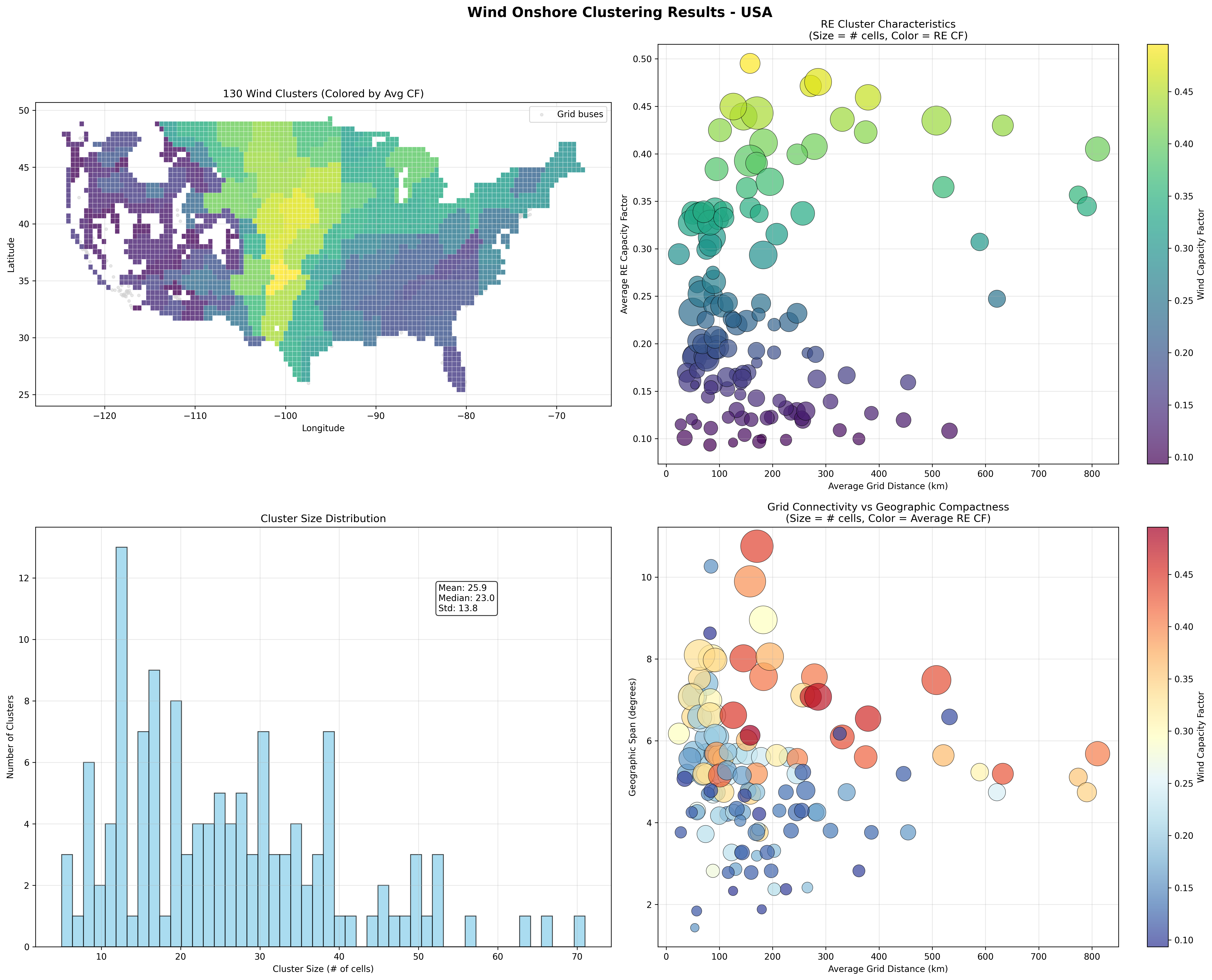
USA Onshore Wind Clustering Results — USA Onshore Wind Resource Clustering - CIT Grid Definition

3,109 renewable grid cells processed
139 clusters created (using dynamic scaling: 3,109^0.6 ≈ 139)
Average cluster size: 22.4 grid cells per cluster
Onshore wind capacity factor: 17.1% to 29.3% range (average 22.8%)
Grid connectivity: Distance to cities (CIT grid)
Cluster size range: 4 to 68 grid cells per cluster

China Solar Clustering (CIT Grid)

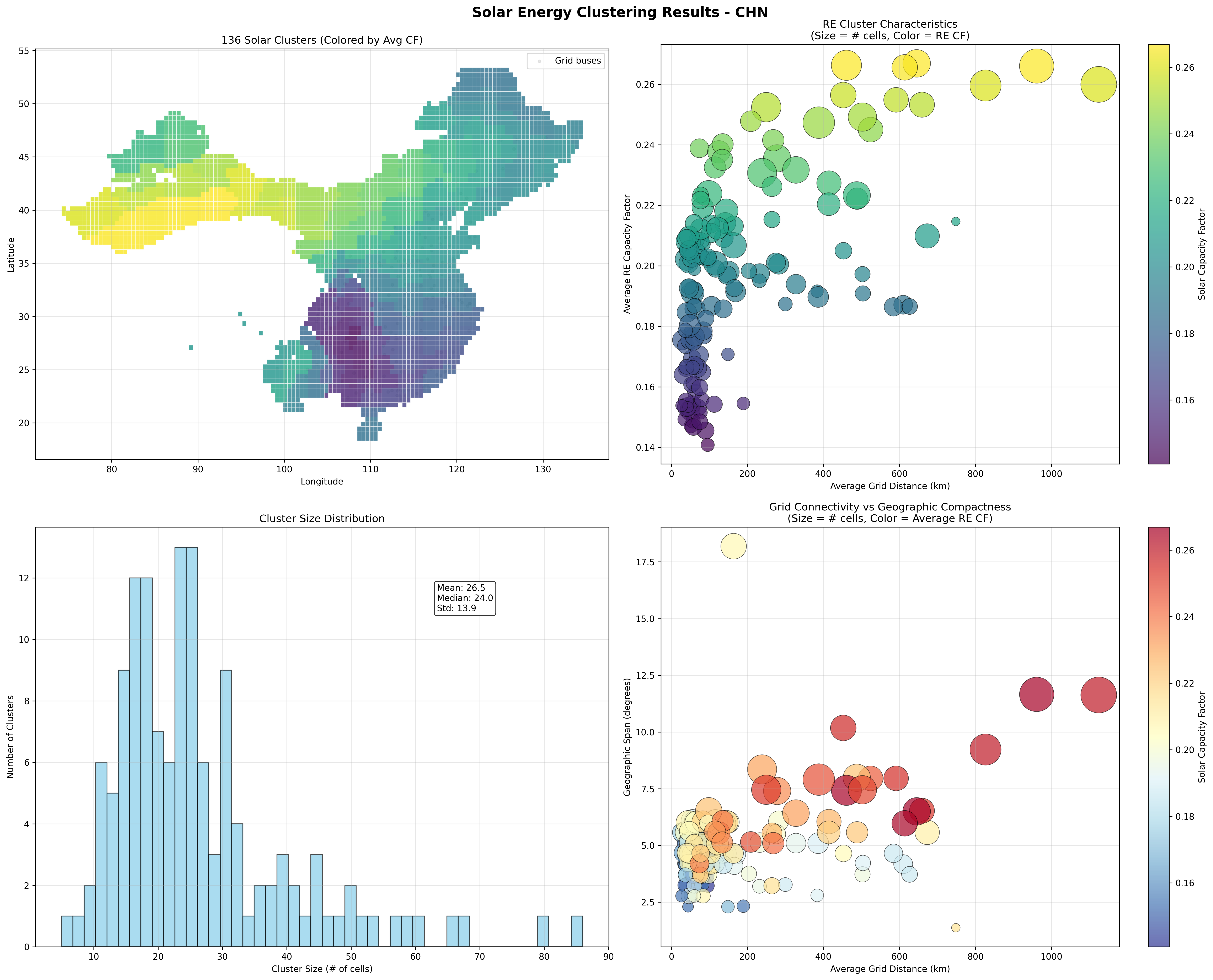
China Solar Clustering Results — China Solar Resource Clustering - CIT Grid Definition

4,047 renewable grid cells processed
165 clusters created (using dynamic scaling: 4,047^0.6 ≈ 165)
Average cluster size: 24.5 grid cells per cluster
Solar capacity factor: 11.2% to 21.8% range (average 16.2%)
Grid connectivity: Distance to cities (CIT grid)
Cluster size range: 3 to 89 grid cells per cluster

China Onshore Wind Clustering (CIT Grid)

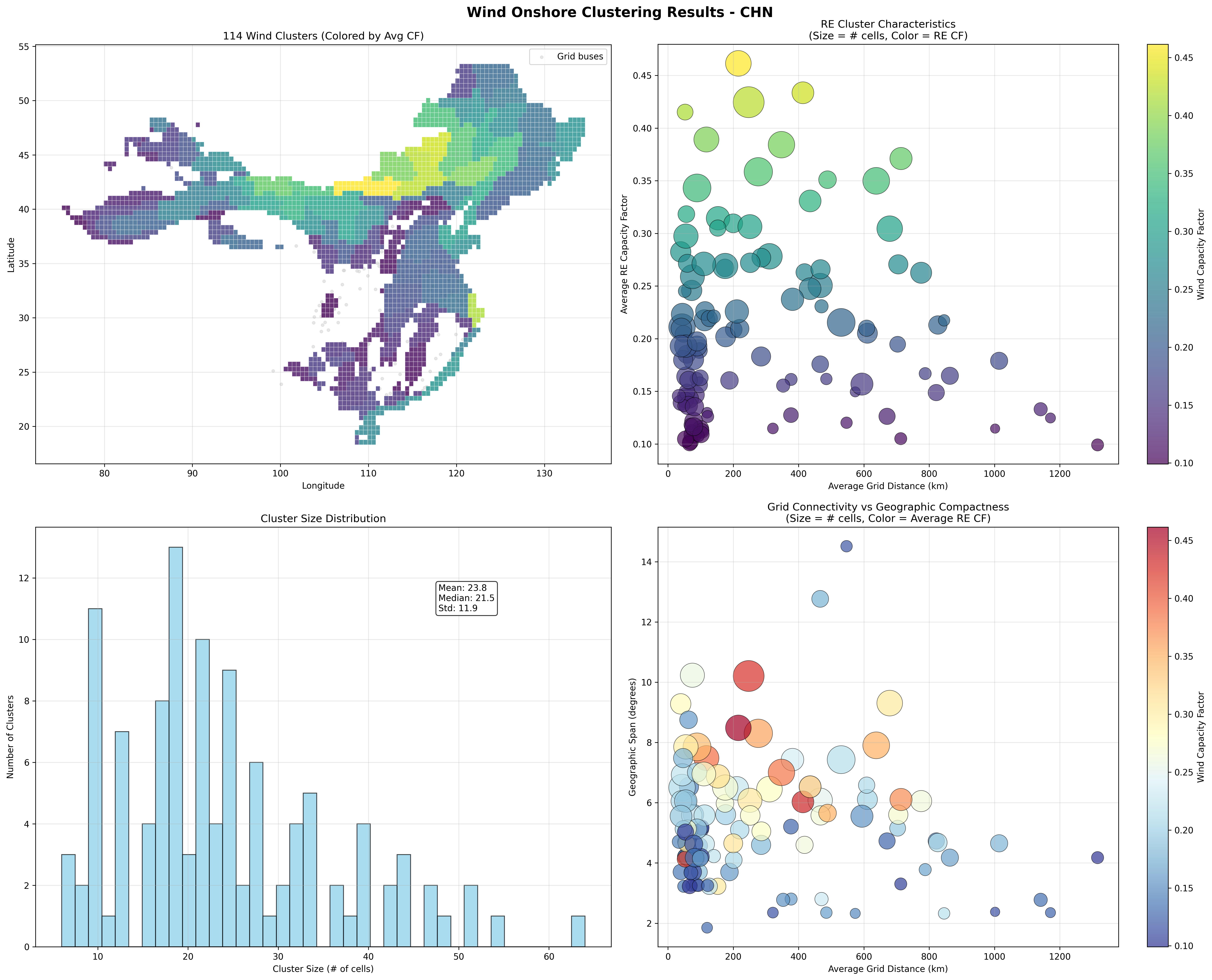
China Onshore Wind Clustering Results — China Onshore Wind Resource Clustering - CIT Grid Definition

4,047 renewable grid cells processed
165 clusters created (using dynamic scaling: 4,047^0.6 ≈ 165)
Average cluster size: 24.5 grid cells per cluster
Onshore wind capacity factor: 15.1% to 35.2% range (average 23.8%)
Grid connectivity: Distance to cities (CIT grid)
Cluster size range: 2 to 97 grid cells per cluster

These examples demonstrate how the clustering methodology adapts to different: - Geographic scales: From Brazil’s focused coastal grid cells to China’s continental expanse - Resource characteristics: Solar vs. wind temporal patterns and capacity factors - Grid definitions: KAN (infrastructure-based) vs. CIT (city-based) transmission proxies - Technology types: Independent clustering for onshore wind, offshore wind, and solar PV

Stage 3: Cluster-Based Renewable Energy Integration

Universal Clustering Approach

VerveStacks applies renewable energy clustering to all model architectures, recognizing that geographic hedging of wind resources and spatial diversity are too important to ignore, regardless of transmission network detail. Both grid and non-grid models use the same clustering methodology from Stage 2, differing only in their approach to synthetic grid definition.

Synthetic Grid Definition

Grid Models: Infrastructure-Based Buses - Data Source: Actual transmission infrastructure from OpenStreetMap - Bus Definition: Physical substations and transmission nodes - Clustering Target: Real transmission buses with known coordinates - Grid Distance: Actual distance to nearest transmission infrastructure

Non-Grid Models: Population and Generation-Based Synthetic Buses - Data Source: Population centers and generation clusters as bus proxies - Bus Definition: Major cities and industrial centers representing demand/supply nodes - Clustering Target: Synthetic buses based on economic activity and generation patterns - Grid Distance: Distance to nearest synthetic bus (population/generation center)

Key Insight: Both approaches result in similar cluster counts (10-300 clusters) and preserve essential geographic diversity for renewable resource hedging.

Cluster-Based Renewable Integration

Universal Methodology:

Technology-Specific Cluster Commodities:

# Each technology gets separate cluster sets
for cluster_id in solar_clusters:
    commodity = f"elc_spv-{iso_code}_{cluster_id:04d}"
    process = f"solar_resource_cluster_{cluster_id}"

for cluster_id in wind_onshore_clusters:
    commodity = f"elc_won-{iso_code}_{cluster_id:04d}"
    process = f"wind_onshore_resource_cluster_{cluster_id}"

for cluster_id in wind_offshore_clusters:
    commodity = f"elc_wof-{iso_code}_{cluster_id:04d}"
    process = f"wind_offshore_resource_cluster_{cluster_id}"

Technology-Specific Capacity-Weighted Temporal Profiles:

# Use technology-specific capacity-weighted cluster profiles
for cluster_id in solar_clusters:
    solar_profile = solar_cluster_profiles[cluster_id]['weighted_cf']
    normalized_solar_profile = solar_profile / solar_profile.sum()

for cluster_id in wind_onshore_clusters:
    wind_profile = wind_cluster_profiles[cluster_id]['weighted_cf']
    normalized_wind_profile = wind_profile / wind_profile.sum()

Technology-Specific Grid Connection Costs:

# Distance-based connection costs calculated separately per technology
for cluster in solar_clusters:
    solar_connection_cost = 1.1 * cluster.avg_grid_dist_km  # M$/GW-km
    solar_transmission_losses = 1 - 0.00006 * cluster.avg_grid_dist_km

for cluster in wind_clusters:
    wind_connection_cost = 1.1 * cluster.avg_grid_dist_km  # M$/GW-km
    wind_transmission_losses = 1 - 0.00006 * cluster.avg_grid_dist_km

Grid Connection Architecture

Grid Models: Direct Bus Connection - Connection: Clusters connect directly to specific transmission buses - Transmission: Explicit network constraints and power flow modeling - Optimization: Location-specific renewable deployment with transmission limits

Non-Grid Models: National Copper Plate Connection - Connection: Clusters connect to national copper plate after paying connection costs - Transmission: No internal transmission constraints (infinite capacity) - Optimization: Technology-level competition with geographic diversity preserved

Economic Integration

Technology-Specific Output Files

The separate clustering approach generates independent output files for each renewable technology:

Solar timeseries: solar_timeseries_<iso_code>.csv and solar_timeseries_<iso_code>.parquet
Wind onshore timeseries: wind_onshore_timeseries_<iso_code>.csv and wind_onshore_timeseries_<iso_code>.parquet
Wind offshore timeseries: wind_offshore_timeseries_<iso_code>.csv and wind_offshore_timeseries_<iso_code>.parquet

Each file contains hourly capacity factor profiles for all clusters of that technology, enabling: - Independent model validation for each renewable type - Technology-specific capacity expansion analysis - Separate temporal pattern analysis (diurnal vs. weather-driven) - Flexible model architecture supporting different renewable integration strategies

Both model architectures incorporate identical economic signals:

Connection Costs: $1.1 million per MW-km based on distance to nearest bus
Transmission Losses: 0.6% per 100 km following industry standards
Geographic Hedging: Wind resource diversity captured through cluster-specific profiles
Capacity Factors: Individual cluster profiles preserve spatial and temporal variations

Output: Multiple commodities per technology with cluster-specific profiles (e.g., elc_spv-USA_0001, elc_spv-USA_0002, …)

Grid vs. NoGrid Comparison:

**Model Architecture Differences**
Aspect	NoGrid Models	Grid Models
Spatial Resolution	Renewable energy clusters (10-300 clusters)	Renewable energy clusters (10-300 clusters)
Renewable Commodities	Multiple per technology (elc_spv-ISO_####)	Multiple per technology (elc_spv-ISO_####)
Temporal Profiles	Capacity-weighted cluster profiles	Capacity-weighted cluster profiles
Synthetic Grid Basis	Population and generation centers	Actual transmission infrastructure
Transmission Modeling	National copper plate (infinite capacity)	Explicit network constraints and power flows
Connection Costs	Distance to synthetic buses	Distance to transmission buses
Use Cases	Policy analysis, scenario studies	Grid integration, network planning
Computational Complexity	Medium (clusters + copper plate)	High (clusters + transmission network)
Geographic Hedging	Preserved through clustering	Preserved through clustering
Economic Dispatch	Technology-level competition with spatial diversity	Location-specific optimization with transmission limits

Data Sources and Integration

Primary Data Sources:

**Renewable Characterization Data Sources**
Data Source	Content & Application
REZoning Database	50×50km grid cell renewable potential (LCOE, capacity factor, suitable area) for 100+ countries. Quality filtering applied: solar PV >5% CF, onshore wind >8% CF
Atlite Weather Data	Hourly capacity factors (8760 hours) for solar PV and wind technologies by grid cell
EMBER Statistics	Base year (2022) renewable generation for demand-constrained resource selection
Global Energy Monitor (GEM)	Existing renewable plant locations for spatial validation and gap-filling
OpenStreetMap (OSM)	Transmission network data for grid model bus-grid cell mapping

Data Processing Pipeline:

Global Land-Use Adjustment: rezoning_landuse_processor.py
ISO-Level Shape Generation: atlite_data_integration.py
Resource Binning: spatial_utils.py - calculate_rez_weights()
Grid Model Integration: grid_modeling.py - compile_solar_wind_data_grid()
Temporal Profile Processing: time_slice_processor.py

Quality Assurance and Validation

Validation Framework:

**Renewable Characterization Quality Controls**
Validation Level	Quality Control Process
Data Consistency	Cross-validation between REZoning, Atlite, and EMBER datasets for coverage and alignment
Physical Constraints	Capacity factors bounded (0-100%), annual normalization verified (±0.001 tolerance)
Economic Rationality	LCOE-based ranking validated against real-world deployment patterns
Spatial Integrity	Grid cell assignments verified against transmission network topology
Temporal Accuracy	Seasonal patterns validated (summer solar peaks, winter wind maxima)

Conservative Assumptions:

Land-Use Reductions: 40% (solar) and 30% (wind) for realistic land availability
Overlap Adjustments: 5-15% typical reduction in total renewable potential
Resource Selection: Demand-constrained rather than full supply curve modeling
Technology Competition: Balanced approach prevents unrealistic monopolization

Innovation Highlights

Key Methodological Innovations:

LCOE-Based Land-Use Conflict Resolution: First implementation of economic rationality in spatial resource allocation
Dual-Architecture Shape Assignment: Seamless switching between national and grid-aware modeling
Demand-Constrained Resource Selection: Realistic alternative to full supply curve evaluation
Conservative Potential Assessment: Addresses over-optimistic renewable resource estimates
Integrated Temporal-Spatial Processing: Unified pipeline from global data to model-ready profiles

Impact on Energy System Modeling:

Realistic Resource Assessment: Conservative potentials improve model credibility
Economic Dispatch Accuracy: LCOE-based allocation reflects real-world deployment
Grid Integration Analysis: High-resolution spatial modeling enables transmission planning
Computational Efficiency: Demand-constrained selection reduces model complexity
Technology Neutrality: Data-driven approach eliminates modeling bias

This comprehensive renewable characterization methodology ensures that VerveStacks energy system models accurately represent the spatial, temporal, and economic dimensions of renewable energy resources while maintaining computational tractability for policy analysis and energy system planning.